What Is Standard Deviation? Variance, n vs n−1, and a Worked Example
Standard deviation (SD) tells you how far values typically sit from their mean, in the same unit as the data: a small SD means the values cluster tightly around the average, a large one means they are spread out. To calculate it, subtract the mean from each value, square those deviations, average the squares to get the variance, and take the square root. Divide by n when your numbers are the entire group you care about (Excel’s STDEV.P) and by n − 1 when they are a sample standing in for a larger group (STDEV.S).
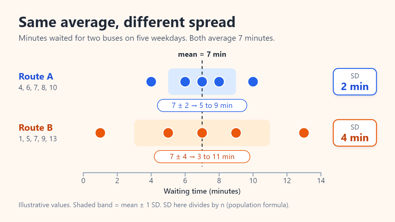
Same average, different spread
Imagine logging how long you waited for two buses on five weekdays (illustrative numbers). Route A: 4, 6, 7, 8 and 10 minutes. Route B: 1, 5, 7, 9 and 13 minutes. Both average exactly 7 minutes, so the mean alone says the routes are identical. They are not: Route A is predictable, while Route B swings from 1 minute to 13.
Standard deviation puts a number on that difference. Route A’s SD is 2 minutes and Route B’s is 4 minutes, so Route B’s waits are spread twice as widely around the same average. Strictly, the SD is a root-mean-square distance rather than a plain average distance, so it gives extra weight to values far from the mean.
How to calculate standard deviation step by step
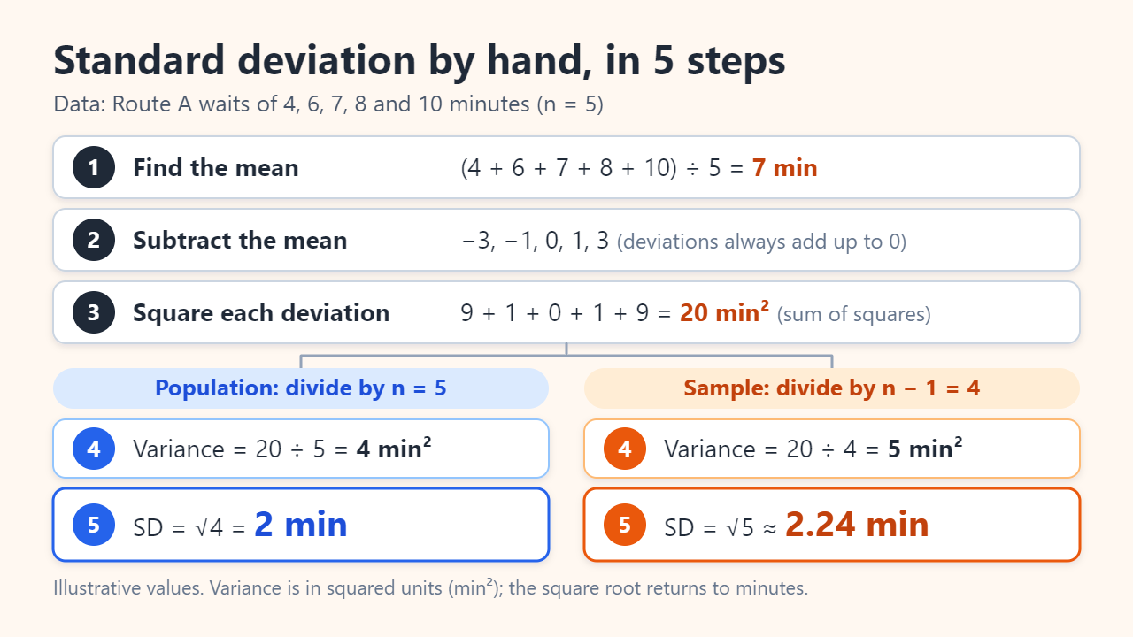
- Find the mean. (4 + 6 + 7 + 8 + 10) ÷ 5 = 35 ÷ 5 = 7 minutes.
- Subtract the mean from each value. The deviations are −3, −1, 0, 1 and 3. They always add up to zero, which is why you cannot simply average them.
- Square each deviation. 9, 1, 0, 1 and 9. Squaring removes the minus signs. Their total, 20, is called the sum of squares.
- Divide to get the variance. 20 ÷ 5 = 4 if the five days are the whole data set you care about (population), or 20 ÷ 4 = 5 if they are a sample (explained below).
- Take the square root. √4 = 2 minutes, or √5 ≈ 2.24 minutes.
| Wait (min) | Deviation from 7 | Squared deviation (min²) |
|---|---|---|
| 4 | −3 | 9 |
| 6 | −1 | 1 |
| 7 | 0 | 0 |
| 8 | 1 | 1 |
| 10 | 3 | 9 |
| Sum: 35 | 0 | 20 |
Route B works the same way: deviations −6, −2, 0, 2 and 6; squares summing to 80; 80 ÷ 5 = 16; SD = √16 = 4 minutes.
Variance vs standard deviation: why square, then take the root?
Variance is essentially the average squared deviation, and standard deviation is its square root. They carry the same information in different units. Route A’s variance is 4 “square minutes,” which is hard to picture; its SD is 2 minutes, which you can compare directly with the 7-minute mean. NIST’s Engineering Statistics Handbook puts it the same way: the square root restores the original units.
Why square in the first place? Positive and negative deviations cancel out, so something has to remove the signs. Squaring does that and also makes large deviations count more. Averaging the absolute deviations instead (the mean absolute deviation) gives 8 ÷ 5 = 1.6 minutes for Route A, smaller than the SD of 2 because the SD leans harder on the ±3 values. Variance stays popular because its math is convenient: the variances of independent quantities simply add.
- Report the SD when people need to read the spread in real units such as minutes, points or kilograms.
- Work with variance inside formulas, models and statistical tests, where adding and splitting variances is easier.
Population (n) vs sample (n − 1): which formula to use
The divisor depends on your question, not on the numbers. If the five days are all you want to describe (“how did my waits go last week?”), they are a population: divide by n and use the symbol σ. If you use them to judge how Route A usually behaves, they are a sample from a much larger set of days: divide by n − 1 and use the symbol s.
The n − 1 rule is called Bessel’s correction. Deviations in a sample are measured from the sample’s own mean, which by construction sits in the middle of those particular values, so they come out slightly smaller than deviations from the true, unknown mean. Dividing by n would therefore underestimate the variance on average, by a factor of (n − 1)/n; dividing by n − 1 removes that bias.
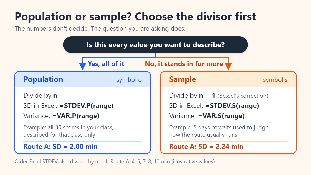
| Item | Population | Sample |
|---|---|---|
| Divide the sum of squares by | n | n − 1 |
| Usual symbol | σ | s |
| Excel SD function | STDEV.P | STDEV.S (older: STDEV) |
| Excel variance function | VAR.P | VAR.S |
| Route A result | 2.00 min | 2.24 min |
In Excel, with the five waits in A2:A6, =STDEV.P(A2:A6) returns 2 and =STDEV.S(A2:A6) returns about 2.236. Per Microsoft’s documentation, both ignore empty cells, text and logical values in a referenced range, so numbers stored as text silently drop out.
How much does the choice matter?
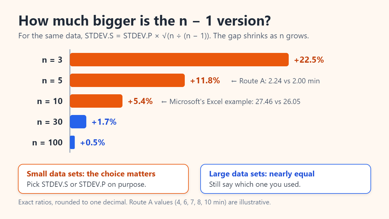
For the same data, the sample SD is larger by a factor of √(n ÷ (n − 1)). That works out to 22.5% larger at n = 3, 11.8% at n = 5, 5.4% at n = 10, 1.7% at n = 30 and only 0.5% at n = 100. Microsoft’s own 10-value example shows the n = 10 case: STDEV.S returns 27.46 and STDEV.P returns 26.05.
How to read standard deviation in practice
Read an SD next to its mean and unit. A 2-minute SD on a 7-minute average is a lot of relative variation; the same 2 minutes on a 60-minute commute is very little. Dividing the SD by the mean (the coefficient of variation) makes this explicit: 2 ÷ 7 ≈ 29% for Route A and 4 ÷ 7 ≈ 57% for Route B.
When data are roughly bell-shaped (normally distributed), the SD also tells you where most values fall. According to NIST, 68.27% of a normal population lies within ±1 SD of the mean, 95.45% within ±2 SD and 99.73% within ±3 SD. For bell-shaped exam scores with a mean of 70 and an SD of 10 (illustrative), about two-thirds would fall between 60 and 80. The rule does not hold for skewed data such as incomes or waiting times with long tails.
Common mistakes
- Using STDEV.P on a small sample. It understates the spread: at n = 5, STDEV.S comes out 11.8% higher.
- Reporting variance as if it were the SD. A variance of 4 min² is an SD of 2 minutes, not 4.
- Ignoring outliers. Because deviations are squared, one extreme value can dominate. Change Route A’s 10 to 20 and its population SD jumps from 2 to about 5.66 minutes.
- Applying the 68–95–99.7 rule to skewed data. Look at a histogram before you use it.
- Confusing SD with standard error. The standard error of the mean, s ÷ √n, describes how precisely the average is known, not how spread out individual values are. For Route A it is 2.24 ÷ √5 ≈ 1.0 minute.
FAQ
Can standard deviation be negative?
No. It is the square root of an average of squares, so the smallest possible value is 0, which happens only when every value is identical.
Is standard deviation the same as the average deviation?
No. The mean absolute deviation averages the distances themselves, while the SD averages squared distances and then takes the root. For Route A they are 1.6 and 2 minutes.
Which should I use for my class’s test scores?
To describe only that class, use STDEV.P. To treat the class as a sample of students in general, use STDEV.S.
Sources: NIST e-Handbook: Measures of Scale; NIST e-Handbook: What do we mean by “Normal” data?; Microsoft Support: STDEV.S function; Microsoft Support: STDEV.P function
Related reading
Original illustrations created to help explain this article.