Documents and work tools · 10/14/2026 · Updated 10/15/2026

Excel #N/A, #VALUE!, #REF!, #DIV/0! and #NAME? Errors: Causes and Fixes

Each Excel error value names a specific problem. #N/A means a lookup found no match, #VALUE! means a formula got the wrong kind of data (often text or a hidden space), #REF! means a referenced cell no longer exists, #DIV/0! means the divisor is zero or blank, and #NAME? means Excel doesn't recognize a word in the formula. Fix the cause first, and wrap a formula in IFNA or IFERROR only when the error is expected, such as a code that genuinely isn't in your list.

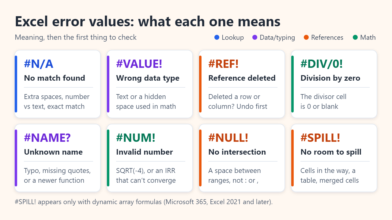
Cheat sheet of eight Excel error values with their meaning and first check: #N/A no match found, #VALUE! wrong data type, #REF! reference deleted, #DIV/0! division by zero, #NAME? unknown name, #NUM! invalid number, #NULL! no intersection, #SPILL! no room to spill — Figure 1. Each error code points to one kind of problem, so the code itself tells you what to check first.

Excel error values at a glance

Microsoft documents seven classic error values, plus #SPILL! for dynamic array formulas in Microsoft 365 and Excel 2021 or later. Read the code before you read the formula: it tells you where to look.

Error	What Excel is saying	Typical trigger	First fix
#N/A	No value is available	A lookup value is not found	Check spaces, data types and exact match
#VALUE!	Wrong kind of data	Math on text, or on a cell holding a space	Clean the cell; use SUM instead of +
#REF!	Invalid cell reference	A referenced row or column was deleted	Undo, or rebuild the reference
#DIV/0!	Division by zero	The divisor is 0 or blank	Test the divisor with IF
#NAME?	Unrecognized text	Misspelled function, unquoted text, unknown name	Fix the spelling or add quotes
#NUM!	Invalid numeric value	SQRT of a negative; IRR finds no result	Fix the input or try another guess
#NULL!	Ranges do not intersect	A space between two ranges	Use a colon or a comma
#SPILL!	Results cannot be placed	Cells in the spill range are not empty	Clear or move the blocking cells

For a stubborn case, select the cell and choose Formulas > Evaluate Formula (in the Formula Auditing group). It steps through the calculation one part at a time and shows exactly where the error first appears.

#N/A: the lookup found no match

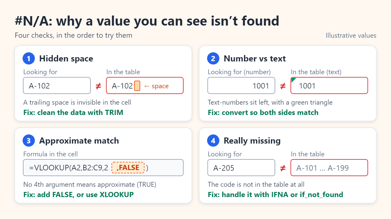
With VLOOKUP, XLOOKUP, MATCH or XMATCH, #N/A means Excel searched and found nothing equal to the lookup value. When you can see the value in the table, the two entries usually differ in a way you can't see. Work through these checks in order:

Hidden spaces. "A-102 " with a trailing space is not "A-102". TRIM removes extra spaces, but not the nonbreaking space (character 160) that often comes with text pasted from web pages; replace it first with SUBSTITUTE(A2,CHAR(160)," ").
Number vs text. The number 1001 does not match the text "1001". Numbers stored as text usually sit left-aligned with a small green triangle. Convert one side so both are numbers or both are text.
Approximate match. If you leave out VLOOKUP's last argument, it defaults to TRUE (approximate match), which can return #N/A or the wrong row on unsorted data. Add FALSE. XLOOKUP matches exactly by default.
Really missing. If the code isn't in the table, the error is telling the truth. Decide what should appear instead and handle it on purpose, as described in the IFNA section below.

Four panels explaining #N/A in lookups: a hidden trailing space after A-102, the number 1001 versus the text 1001, VLOOKUP without FALSE doing an approximate match, and a code A-205 that is really missing — Figure 2. When a lookup returns #N/A for a value you can see, rule out hidden spaces, number-versus-text mismatches and approximate matching before deciding the value is missing.

#VALUE! and #NAME?: wrong data and unrecognized text

#VALUE! appears when a formula can't use the data it was given. The classic case is arithmetic on a cell that looks empty but holds a space, or on a number typed with a stray character. Operators such as + and * fail on text, while functions such as SUM skip it, so Microsoft suggests =SUM(A2:C2) instead of =A2+B2+C2. Evaluate Formula exposes the culprit: a hidden space shows up as " ".

#NAME? means Excel doesn't recognize something you typed. The usual suspects:

A misspelled function, such as =VLOKUP(...). Picking functions from the autocomplete list prevents this.
Text without double quotes: =IF(A2>B2,"Over","OK") works, but leaving out the quotes around Over does not.
A defined name that doesn't exist or is misspelled. Check Formulas > Name Manager.
A newer function, such as XLOOKUP, opened in an older version of Excel that doesn't include it.

#REF! and #DIV/0!: missing references and empty divisors

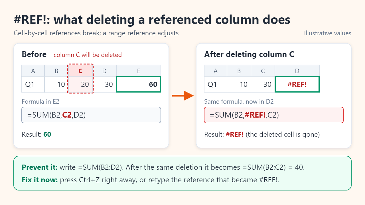
#REF! means a formula points at a cell that no longer exists. In Microsoft's own example, =SUM(B2,C2,D2) becomes =SUM(B2,#REF!,C2) once column C is deleted. Press Ctrl+Z right away to bring the column back; if it's too late, retype the broken reference. Prevention is easier: =SUM(B2:D2) shrinks to =SUM(B2:C2) when a column inside the range is deleted, so it keeps working.

Before and after deleting column C: =SUM(B2,C2,D2) showing 60 becomes =SUM(B2,#REF!,C2) showing #REF!, while the range form =SUM(B2:D2) would become =SUM(B2:C2) and show 40 — Figure 3. Deleting a column that a formula names cell by cell produces #REF!; a range reference adjusts instead (illustrative values).

#REF! also appears when VLOOKUP's column number is larger than the table, such as asking for column 5 of a four-column range, and when INDIRECT points to a workbook that is closed.

#DIV/0! means the divisor is 0 or an empty cell, which often happens in rows where data hasn't been entered yet. Test the divisor first: =IF(C2,B2/C2,"") stays blank while C2 is empty or zero and divides once a value arrives. Watch AVERAGEIF too, because it returns #DIV/0! when no cells meet the criteria.

#NUM!, #NULL! and #SPILL!: the less common three

#NUM!: a numeric argument is invalid or no result can be found. =SQRT(-4) returns it, and IRR returns it when it can't find a result after 20 tries; Microsoft suggests trying a different guess value.
#NULL!: a space between two references is Excel's intersection operator. =SUM(A1:A5 C1:C5) asks for the cells both ranges share, and there are none. Use a comma for separate ranges, =SUM(A1:A5,C1:C5), or a colon for one continuous block.
#SPILL!: a dynamic array formula such as FILTER, UNIQUE or SORT returns several results but can't place them. Usually something already sits in the spill range: select the error cell, open the warning icon and choose Select Obstructing Cells. Spilled formulas also fail inside Excel tables, over merged cells, and when a whole-column reference would run past the bottom of the sheet.

IFERROR vs IFNA: when hiding an error is acceptable

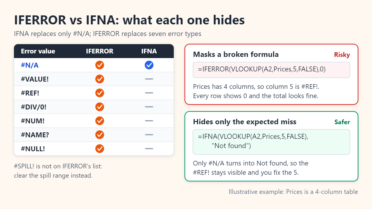
Both functions take a formula and a replacement value. IFERROR(value, value_if_error) replaces seven error types: #N/A, #VALUE!, #REF!, #DIV/0!, #NUM!, #NAME? and #NULL!. IFNA(value, value_if_na) replaces only #N/A. #SPILL! isn't on IFERROR's list, and wrapping a blocked formula doesn't give its results anywhere to go, so clear the spill range instead.

The difference matters. Take a four-column price table and the illustrative formula =IFERROR(VLOOKUP(A2,Prices,5,FALSE),0). Column 5 doesn't exist, so every row quietly shows 0 and the total still looks plausible. With IFNA in place of IFERROR, the #REF! stays on screen and you correct the column number.

Table showing IFERROR replaces #N/A, #VALUE!, #REF!, #DIV/0!, #NUM!, #NAME? and #NULL! while IFNA replaces only #N/A, with an example where IFERROR turns a #REF! into 0 and IFNA leaves it visible — Figure 4. IFERROR hides seven error types, IFNA only #N/A. Wrapping a lookup in IFNA keeps real formula mistakes visible.

Practical rules:

Get the formula working first. Microsoft warns that blanket error handlers suppress every error, not just the one you expect.
For lookups, handle the missing case with IFNA or XLOOKUP's if_not_found argument so other errors stay visible.
Prefer a visible label such as "Not found" over 0. A zero looks like real data and drags down averages.
Keep IFERROR for display cells where any error means the same thing, and test the formula before wrapping it.

FAQ

Is ##### an error?

Not a formula error. It usually means the column is too narrow to show the number or date, so widen it. It also appears when a cell holds a negative date or time value.

Why does a workbook show #NAME? only on a colleague's computer?

Their Excel probably lacks a function the workbook uses. Microsoft notes that newer functions return #NAME? when recalculated in earlier versions. Swap in an older equivalent, or open the file in a version that includes the function.

What does the small green triangle in a cell mean?

It's background error checking flagging a possible problem, such as a number stored as text or a formula that differs from its neighbors. It isn't an error value. You can turn individual rules on or off under File > Options > Formulas.

Sources: Microsoft Support: Detect formula errors in Excel; Microsoft Support: How to correct a #REF! error; Microsoft Support: IFERROR function; Microsoft Support: IFNA function