XLOOKUP in practice: find an item by code and handle missing matches
This article was translated from its source language with AI assistance. Please check technical terms and equations against the original.
Build a small worksheet that retrieves an item name when you enter its code. XLOOKUP separates the value to find, the range to search, and the range to return. Start with one straightforward formula and test a present value, a missing value, and a duplicate before introducing more complicated formulas.
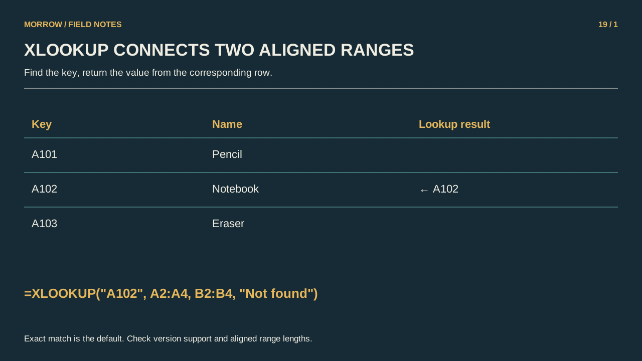
Find an exact match in a three-row table
Put Code in A1 and Item in B1. Enter the following records in A2:B4, then type A102 in E2. The example values are fictional and deliberately small enough to check by eye.
| Row | A: Code | B: Item |
|---|---|---|
| 2 | A101 | Pencil |
| 3 | A102 | Notebook |
| 4 | A103 | Eraser |
=XLOOKUP(E2,$A$2:$A$4,$B$2:$B$4,"Not found",0)The result is Notebook. The final zero requests exact matching. Exact matching is also the default, but stating it makes this example's intention clear. Dollar signs keep the reference table fixed when the formula is copied down, while E2 can move to E3 for the next input.
Missing codes and duplicate codes are different problems
Change E2 to A999 and the result becomes Not found. This is handling a normal missing match, not hiding every possible formula error. Returning zero for a missing code can be confusing when zero is also a valid result, so choose a missing-value representation that suits the returned data.
If A102 occurs twice, the default search returns the first match. It does not add the records or decide which one is newest. If product codes must be unique, inspect duplicates in the source. Searching from the bottom is a separate option, and it only means latest when the row order really represents time.
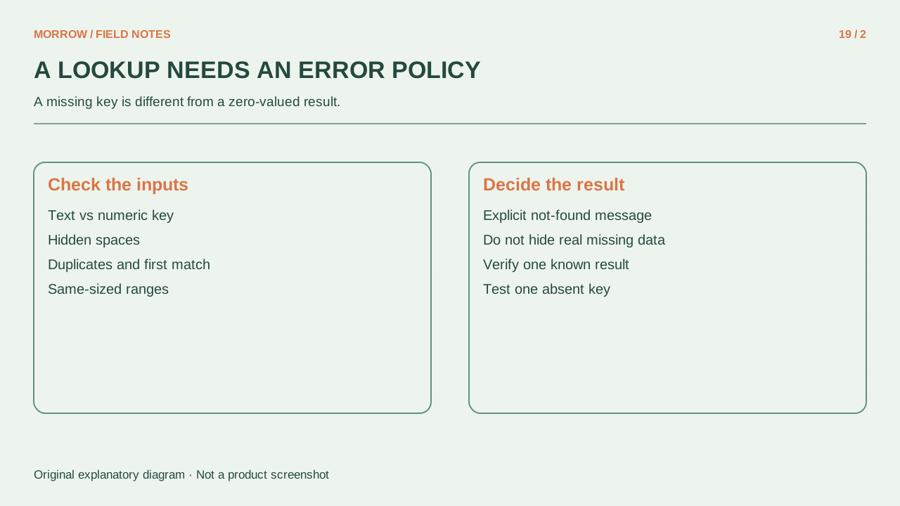
Inspect data as well as ranges when a match fails
- Check that lookup and return ranges cover corresponding rows and have compatible sizes.
- Check whether a code is numeric in one place and text in another.
- Inspect leading or trailing spaces and unwanted source characters.
- Understand the source's identifier rules before normalizing values.
Automatically turning text 00123 into numeric 123 may merge two different products. A failed lookup suggests a data check; it is not permission to change the meaning of an identifier. Also do not treat an ordinary XLOOKUP as a case-sensitive identifier validation system. If that distinction is required, design a separate check for it.
Use a compatible alternative for older workbooks
XLOOKUP is unavailable in Excel 2016 and 2019. Check a supported version such as Microsoft 365, Excel 2021, or Excel 2024 before sharing the workbook. This simple example can use INDEX with exact-match MATCH instead:
=INDEX($B$2:$B$4,MATCH(E2,$A$2:$A$4,0))The alternative returns #N/A for a missing code, so decide on missing-value handling separately. Adding every quantity for one code is another task; use SUMIF or SUMIFS when a total is required. Test A102, A999, and a duplicate A102 in a disposable sheet before applying the lookup to important records.
Primary references: Microsoft XLOOKUP, MATCH, and INDEX. Regional settings may require semicolons instead of commas as argument separators.
Related practical guides
Original illustrations created to help explain this article.